Topics

History of the Ozone Hole

Throughout the 20th century, discoveries and observations trickled in that would allow scientists to understand how human-made chemicals like chlorofluorocarbons create a hole in the ozone layer over Antarctica each spring.

As early as 1912, Antarctic explorers recorded observations of unusual veil-type clouds in the polar stratosphere, although they could not have known at the time how significant those clouds would become. In 1956, the British Antarctic Survey set up the Halley Bay Observatory on Antarctica in preparation for the International Geophysical Year (IGY) of 1957. In that year, ozone measurements using a Dobson Spectrophotometer began.

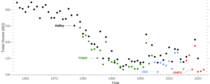
Graph of Antarctic ozone concentrations measured by ground instruments at Halley and from the satellites

Instruments on the ground (at Halley) and high above Antarctica (Total Ozone Mapping Spectrometer [TOMS], Ozone Monitoring Instrument [OMI], and Ozone Mapping and Profiler Suite [OMPS]) measured an acute drop in total atmospheric ozone during October in the early and middle 1980s. (Halley data supplied by J. D. Shanklin, British Antarctic Survey ).

These measurements gave the first clues that there was trouble in the ozone layer. In 1985, a group of scientists (J. C. Farman, B. G. Gardiner, and J. D. Shanklin) published in the journal Nature the first paper on observations of springtime losses of ozone over Antarctica. In 1986, NASA scientists used satellite data from the Total Ozone Mapping Spectrometer (TOMS) and the Solar Backscatter Ultraviolet (SBUV) instrument to demonstrate that the ozone hole is a regional-scale Antarctic phenomenon.

Between 1986 and 1987, several papers suggested possible mechanisms for the ozone hole, including chemical, dynamical (meteorological), and solar cycle influences. Among the key papers explaining the atmospheric chemistry of CFCs and ozone depletion was one by Susan Solomon and several colleagues. The paper also emphasized the need for polar stratospheric clouds to explain the reaction chemistry. Also in 1986, Michael B. McElroy and colleagues described a role for bromine in ozone-depleting reactions. Paul Crutzen and Frank Arnold proposed that the polar stratospheric clouds could be made of nitric acid trihydrate, which would explain the clouds’ presence at an altitude and temperature that should not have been cold enough for the tiny amount of pure water vapor present in the stratosphere to condense.

Observational evidence of the role of chlorine in ozone loss continued to mount during that same period. For example, the National Ozone Expedition (NOZE) measured elevated levels of the chemical chlorine dioxide (OClO) during the springtime ozone hole from McMurdo Research Station. Then in 1987, the Antarctic Airborne Ozone Expedition flew the ER-2 and DC-8 research aircraft from Punta Arenas, Chile, into the Antarctic Vortex.

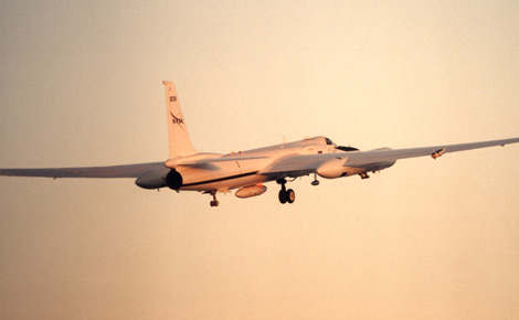
Photograph of a NASA ER-2 lifting off from Kiruna, Sweden to study polar ozone

Aircraft measurements in the late 1980s confirmed the link between CFCs, chlorine, and ozone loss. Here a NASA ER-2 high-altitude research aircraft lifts off from Kiruna, Sweden on a mission to study Arctic ozone. (NASA Dryden Flight Research Center photo EC00-0037-22)

The aircraft observations produced the “smoking gun” linking CFC-derived chlorine to the ozone hole. The flight data showed a negative correlation between chlorine monoxide (ClO) and ozone: the higher the concentration of ClO, the lower the concentration of ozone. In 1988, the husband and wife team Mario and Luisa Molina described the chemical reactions through which ClO catalyzes the extremely rapid destruction of ozone.

NASA has been monitoring the status of the ozone layer through satellite observations since the 1970s, beginning with the TOMS sensors on the Nimbus satellites. The latest-generation ozone-monitoring technology, the Ozone Mapping and Profiler Suite (OMPS), is flying onboard the NASA/NOAA Suomi NPP satellite.